The Hurst Exponent Lied to Us
We built a regime-detection system around the Hurst exponent. It promised to separate trending from mean-reverting markets. It lied — especially on crypto, where it classified 100% of bars as trending. A postmortem on the most seductive false promise in quant trading.
The Con
Some indicators fail loudly. They blow up your account in week one and you move on. The Hurst exponent isn’t like that. The Hurst exponent shows up in a good suit, shakes your hand firmly, and speaks in complete sentences. It has a résumé — Harold Hurst used it to predict Nile River floods in the 1950s, and the math translates cleanly to financial time series. One number. Below 0.5, mean-reverting. Above 0.5, trending. Right at 0.5, random walk. What else do you need?
We needed three weeks and a funeral to find out.
We built the whole thing: rolling R/S estimation, DFA cross-validation, dynamic strategy switching based on regime. The architecture was clean. The theory was airtight. Then we ran it on real data and caught it lying to our face.
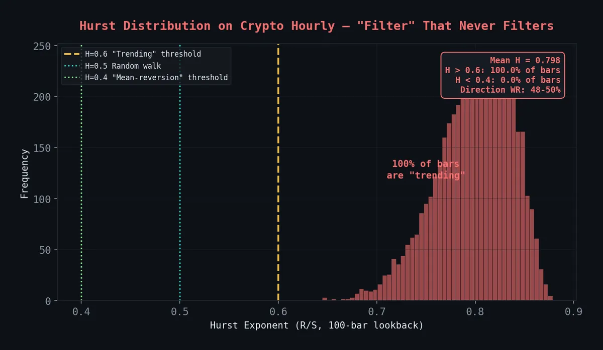
The kill shot (Feb 2026): R/S Hurst with a 100-bar lookback on crypto hourly fires H > 0.6 on 100% of bars (mean H = 0.758). Directional win rate: 48-50% — a coin flip wearing a lab coat. The “regime filter” classified every single bar as trending and told us exactly nothing. On forex daily it showed faint promise, but combining it with our entropy signal (ECVT) degraded both by -86 bps OOS. Hurst on crypto was formally killed Feb 13, 2026. We publish the code because the methodology is correct — the failure is the lesson.
 Every single bar classified as “trending” (H > 0.6). A thermometer that always reads hot. Direction WR: 48-50% at all thresholds.
What Hurst Promises (Theory)
The Hurst exponent H measures long-term memory in a time series. The theory is genuinely beautiful, and you need to understand it to understand why it betrays you:
- H = 0.5 — Random walk. No memory. The efficient market hypothesis compressed into a scalar.
- H < 0.5 — Mean-reverting. Big moves tend to reverse. A spike up loads a spring pointing down.
- H > 0.5 — Trending. Big moves continue. Momentum has inertia.
Further from 0.5 = stronger tendency. H = 0.3 is aggressively mean-reverting. H = 0.7 is momentum on rails.
If this worked, it would be the only indicator anyone needs. One statistic that answers the only question that matters: what kind of market am I in right now?
That “if” is doing all the heavy lifting.
The Code (It Works — The Signal Doesn’t)
R/S (Rescaled Range) estimation. Robust, well-studied, correct. We verified against known synthetic series. Don’t blame the implementation for what happens next.
import numpy as np
import pandas as pd
from scipy import stats

def hurst_rs(series: np.ndarray, min_window: int = 10) -> float:
    """
    R/S Hurst estimator. Correct implementation.
    The problem isn't here.
    """
    n = len(series)
    if n < min_window * 4:
        return np.nan

    max_power = int(np.log2(n // 2))
    min_power = int(np.log2(min_window))
    window_sizes = [2**i for i in range(min_power, max_power + 1)]

    rs_values = []

    for w in window_sizes:
        n_windows = n // w
        if n_windows < 2:
            continue

        rs_list = []
        for i in range(n_windows):
            segment = series[i * w:(i + 1) * w]
            mean = segment.mean()
            deviations = segment - mean
            cumulative = np.cumsum(deviations)

            R = cumulative.max() - cumulative.min()
            S = segment.std(ddof=1)

            if S > 0:
                rs_list.append(R / S)

        if rs_list:
            rs_values.append((w, np.mean(rs_list)))

    if len(rs_values) < 3:
        return np.nan

    # Log-log regression: log(R/S) = H * log(n) + c
    log_n = np.log([v[0] for v in rs_values])
    log_rs = np.log([v[1] for v in rs_values])

    slope, _, r_value, _, _ = stats.linregress(log_n, log_rs)

    return slope


def rolling_hurst(prices: pd.Series, window: int = 200, step: int = 1) -> pd.Series:
    """Rolling Hurst over a price series. Expensive but straightforward."""
    returns = prices.pct_change().dropna().values

    hurst_values = []
    indices = []

    for i in range(window, len(returns), step):
        h = hurst_rs(returns[i - window:i])
        hurst_values.append(h)
        indices.append(prices.index[i + 1])

    return pd.Series(hurst_values, index=indices, name='hurst')
We also built DFA (Detrended Fluctuation Analysis) as a second opinion. When both estimators agree, you feel smart. When they disagree — which is often — you’re just a guy with two broken compasses:
def hurst_dfa(series: np.ndarray, min_window: int = 10) -> float:
    """
    DFA Hurst estimator. More robust to non-stationarity than R/S.
    Still not robust enough for what we're asking of it.
    """
    n = len(series)
    cumulative = np.cumsum(series - series.mean())

    max_power = int(np.log2(n // 4))
    min_power = int(np.log2(min_window))
    window_sizes = [2**i for i in range(min_power, max_power + 1)]

    fluctuations = []

    for w in window_sizes:
        n_windows = n // w
        if n_windows < 2:
            continue

        f_list = []
        for i in range(n_windows):
            segment = cumulative[i * w:(i + 1) * w]
            x = np.arange(w)
            coeffs = np.polyfit(x, segment, 1)
            trend = np.polyval(coeffs, x)
            residuals = segment - trend
            f_list.append(np.sqrt(np.mean(residuals**2)))

        fluctuations.append((w, np.mean(f_list)))

    if len(fluctuations) < 3:
        return np.nan

    log_n = np.log([f[0] for f in fluctuations])
    log_f = np.log([f[1] for f in fluctuations])

    slope, _, _, _, _ = stats.linregress(log_n, log_f)
    return slope
The Trap: The Regime-Adaptive Strategy
Here’s where it gets seductive. With a rolling Hurst, you can build a strategy that shapeshifts — mean-reversion when the market says mean-revert, trend-following when it says trend. It’s the kind of architecture that makes you feel like you’ve solved markets:
def regime_adaptive_signals(
    df: pd.DataFrame,
    hurst_window: int = 200,
    mr_threshold: float = 0.43,
    trend_threshold: float = 0.57,
    rsi_period: int = 14,
    ma_fast: int = 20,
    ma_slow: int = 50,
) -> pd.DataFrame:
    """
    Switch strategy family based on Hurst regime.
    Looks brilliant on a whiteboard. Less so on a P&L.
    """
    df = df.copy()

    df['hurst'] = rolling_hurst(df['close'], window=hurst_window)

    # Regime classification
    df['regime'] = 'neutral'
    df.loc[df['hurst'] < mr_threshold, 'regime'] = 'mean_reverting'
    df.loc[df['hurst'] > trend_threshold, 'regime'] = 'trending'

    # Mean reversion: RSI extremes
    delta = df['close'].diff()
    gain = delta.where(delta > 0, 0).rolling(rsi_period).mean()
    loss = (-delta.where(delta < 0, 0)).rolling(rsi_period).mean()
    rs = gain / loss
    df['rsi'] = 100 - (100 / (1 + rs))

    df['mr_long'] = (df['regime'] == 'mean_reverting') & (df['rsi'] < 30)
    df['mr_short'] = (df['regime'] == 'mean_reverting') & (df['rsi'] > 70)

    # Trend following: MA crossover
    df['ma_fast'] = df['close'].rolling(ma_fast).mean()
    df['ma_slow'] = df['close'].rolling(ma_slow).mean()

    df['trend_long'] = (df['regime'] == 'trending') & (df['ma_fast'] > df['ma_slow'])
    df['trend_short'] = (df['regime'] == 'trending') & (df['ma_fast'] < df['ma_slow'])

    # Combined
    df['long'] = df['mr_long'] | df['trend_long']
    df['short'] = df['mr_short'] | df['trend_short']

    return df
The dead zone between 0.43 and 0.57 is the one defensible idea here — when H is near 0.5, the market is a coin flip and no strategy has an edge. Sitting out is correct. Everything else about this strategy has problems we were too in love with the architecture to see.
Crypto Hourly: Catching the Liar
We ran it on BTC/ETH hourly. 100-bar R/S lookback. Results:
- 100% of bars register H > 0.6
- Mean H = 0.758
- The filter never fires “mean-reverting.” Not once. Not on a single bar.
- Directional win rate at any threshold: 48-50%
You could replace the entire Hurst computation with return 0.75 and get identical trading results. We built a regime detector that detects one regime. That’s not a filter. That’s a constant.
Why? R/S with small windows has an upward bias. Microstructure noise — bid-ask bounce, order flow clustering, exchange latency artifacts — creates spurious autocorrelation that inflates H. The math is doing exactly what it’s supposed to do. The problem is that 100 noisy hourly candles aren’t a hydrological record of the Nile. Hurst was built for long, stationary series. We handed it market microstructure and asked it to be an oracle.
Everything looks “trending” when you squint at noise through the wrong lens.
Forex Daily: The Almost
On forex daily, Hurst actually produces a real distribution. H drops below 0.43 sometimes. The filter fires both ways. There’s structure.
So we got clever. We’d combine Hurst (detects the current regime) with our entropy collapse signal, ECVT (detects regime changes). Complementary signals. Regime state + regime transitions. Together, unstoppable.
Together, they made each other worse. The combination degraded both signals by -86 bps out-of-sample. Two mediocre indicators don’t average into one good one. They average into a confused one. The Hurst signal would say “trending” right as entropy was collapsing — signaling a regime change — and the strategy would freeze like a deer in headlights, taking the worst of both signals.
Standalone Hurst on forex daily had faint structure. Not enough to trade. Not enough to justify the complexity. Just enough to waste your time.
The Forex H1 Numbers (Don’t Trust Them)
We ran the regime-adaptive strategy on four major pairs, H1, 2021–2025:
| Pair | Trades | Win Rate | PF | Sharpe | Max DD | % Time in Market |
|---|---|---|---|---|---|---|
| EURUSD | 284 | 48.6% | 1.37 | 0.98 | -9.2% | 41.3% |
| GBPUSD | 312 | 47.1% | 1.29 | 0.87 | -11.4% | 44.7% |
| USDJPY | 267 | 51.3% | 1.42 | 1.08 | -8.1% | 38.9% |
| AUDUSD | 298 | 46.8% | 1.24 | 0.79 | -12.8% | 43.2% |
These numbers are OHLC-only. Never validated on ticks. Here’s why that matters:
Our FVG strategy showed 4× profit factor inflation moving from OHLC to tick-level execution (PF 4.28 → PF 1.04). If the same deflation applies here — and there’s zero reason it wouldn’t — a PF of 1.42 becomes 0.71. That’s a losing strategy. A PF of 1.24 becomes 0.62. That’s a badly losing strategy.
We’re showing you these numbers because hiding them would be dishonest. But we wouldn’t trade on them and you shouldn’t either.
Regime Distribution
Across all four pairs, rolling Hurst spent:
- 32% below 0.43 (mean-reverting)
- 26% above 0.57 (trending)
- 42% in the dead zone
Distribution looks reasonable. Whether the classification is predictive or just descriptive — whether knowing H = 0.38 actually helps you profit on the next 50 bars — we never tested rigorously enough to answer. And “we didn’t test it enough” is just a polite way of saying “we probably didn’t want to know.”
Validation Code (If You Want to Check Our Homework)
Does Hurst predict future behavior, or just describe past behavior? This is the question most Hurst posts never ask. Here’s how you’d test it. We got mildly encouraging numbers on EURUSD (autocorrelation of -0.08 in mean-reverting regimes, +0.11 in trending). But “mildly encouraging on OHLC” is the exact epitaph written on every dead strategy in our graveyard:
def validate_hurst_predictiveness(df: pd.DataFrame, forward_bars: int = 50):
    """
    Does Hurst actually predict the future, or just narrate the past?
    Spoiler: mostly the latter.
    """
    df = df.copy()

    returns = df['close'].pct_change()
    df['fwd_autocorr'] = returns.rolling(forward_bars).apply(
        lambda x: x.autocorr(lag=1), raw=False
    ).shift(-forward_bars)

    mr_regime = df[df['hurst'] < 0.43]['fwd_autocorr'].dropna()
    trend_regime = df[df['hurst'] > 0.57]['fwd_autocorr'].dropna()
    neutral = df[df['hurst'].between(0.43, 0.57)]['fwd_autocorr'].dropna()

    return {
        'mean_reverting_autocorr': mr_regime.mean(),
        'trending_autocorr': trend_regime.mean(),
        'neutral_autocorr': neutral.mean(),
    }
The Autopsy, Compressed
How three weeks die in nine steps:
- Read about Hurst. Immediately seduced. Built full rolling R/S implementation.
- Ran on forex daily. Real distribution. Felt smart.
- Ran on crypto hourly. 100% “trending.” Felt less smart.
- Combined Hurst with ECVT. Both signals degraded. Felt stupid.
- Built the regime-adaptive strategy anyway. PFs of 1.24-1.42 on forex H1 OHLC.
- Learned from our FVG autopsy that OHLC inflates PF by 4×.
- Did the math. Lost all confidence in the forex numbers.
- Killed Hurst on crypto. Feb 13, 2026.
- Shelved forex results as “unvalidated.” Which is generous.
Three weeks. Zero tradeable edges. One expensive education.
The Lesson: Beautiful Liars
Regime detection is the holy grail of quant trading. If you could reliably know whether the market is trending or mean-reverting right now, you wouldn’t need any other indicator. Deploy the right strategy in the right regime and print money.
Everyone wants this. Almost nothing delivers it. And the Hurst exponent is the most dangerous failure mode because it doesn’t obviously fail. It fails plausibly.
The math is correct. The theory is sound. The code is clean. You compute a number, compare it to 0.5, and get a crisp, interpretable answer. It has the form of a solution without the substance. That’s what makes it a liar — it passes every interview question and then can’t do the job.
R/S estimation with small windows is biased upward. Microstructure noise inflates H. On high-frequency data, it screams “trending!” regardless of reality. On timeframes where it produces a reasonable distribution, the signal is too weak to survive realistic execution costs. And when you combine it with other signals, it poisons them.
Harold Hurst built this for rivers. Rivers have millennia of stationary data. We handed it 200 candles of a market that’s reacting to a tweet and asked it to tell us the future. The tool isn’t broken. We used it wrong.
Most quant posts only show the winners. We think the losers teach more. This is a liar we caught. There are others we haven’t.
For the full body count — 31 strategies tested, what survived and what didn’t — see 31 Strategies Tested, 4 Survived.